1. Introduction
We wanted to work on a large, real-world graph data, so we chose a blockchain graph; we were able to make a basic anomaly detection ML model work, but found it difficult to build neither a comprehensive dataset nor a robust graph neural network due to the insufficient capabilities of existing GNNs and the lack of node features.
| Number of nodes | Number of edges | Number of node features | Number of edge features | |
|---|---|---|---|---|
| Twitter [1] | 8.8k | 119k | 0 | 768 |
| eBay-Large [2] | 8.9M | 13.2M | 480 | 0 |
| Ethereum | 160m | 1.7b | 0 | 3 |
Table 1. Real-life graph datasets
Blockchain has emerged to be one of the largest real-life networks, where millions of transactions taking place every day. As rapid as it grew, there were many incidents of hacks and scams on crypto exchanges, bridges, and DApp protocols leading to the loss of billions of dollars. Hence, detecting abnormal or fraudulent activities on a blockchain transaction network is a crucial task, and can be used in various applications.
In this work, we propose Ethereum phishing transaction prediction framework using graph neural network as its detector backbone. Specifically, we build a scalable framework for anomaly detection via subgraph sampling from daily transaction logs, which can be easily updated and utilized in real-time environment.
In the following section, we review the previous studies of anomaly detection on graph data, including financial transaction network. Next, we introduce our anomaly detection framework which consists of training graph data generation and graph neural network classification model. Lastly, we examine the result of our experiments on finding the phishing entities using our framework, and reflect on the findings and limitations of current state of graph neural network specific to applications on financial data.
Related Concepts
Graph
Graph is a fundamental data structure in computer science that consists of a finite set of nodes (also known as vertices) connected by edges. The graph represents a collection of objects or entities, where the nodes represent the objects, and the edges represent the relationships or connections between the objects. Graphs are used to model a wide range of real-world systems and their relationships, such as social networks, transportation networks, financial transaction networks, and more.
Formally, a graph
is a set of vertices(nodes), representing the objects or entities. is a set of edges, representing the connections or relationships between the vertices. Each edge is an unordered pair where and are elements of , indicating that there is a connection between vertex and vertex .
Graphs can be classified into different types based on various properties, such as directed vs. undirected, simple vs. multi, weighted vs. unweighted, and more. They are widely used in various algorithms and applications, including graph traversal, shortest path finding, network analysis, and graph-based machine learning models.
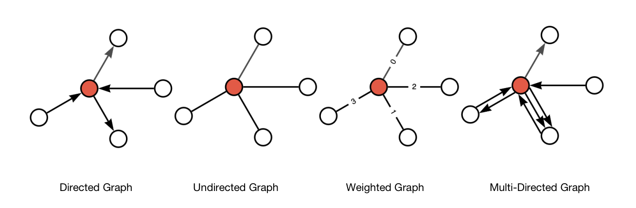
Figure 1. Type of Graphs
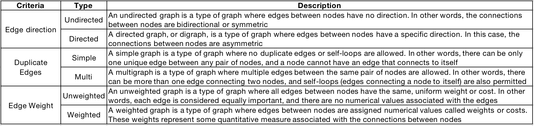
Table 2. Type of Graphs
Learning on Graphs
Working on graphs with machine learning is essentially a process to generate a meaningful representation for the items of interest (nodes, edges, or full graphs), then to use these to train a predictor for the target task. As in other modalities, we want the generated representation of similar objects to be mathematically close.
Before neural networks, walk-based approaches were widely adopted in learning graph representations. These methods use the probability of visiting a node j from a node i on a random walk to define similarity metrics. Node2Vec, for example, simulates random walks between nodes of a graph, then processes these walks with a skip-gram, like we would do with words in sentences, to compute embeddings. However, they cannot obtain embeddings for new nodes, do not capture structural similarity between nodes finely, and cannot use added node or edge features.
Applying the existing deep learning architecture directly to graph data is not a simple task, because graphs are very different from typical objects used in machine learning. Their topology is more complex than just "a sequence" (such as text and audio) or "an ordered grid" (images and videos, for example): in short, their representation is invariable to the orderings.
This leads to a need for a different architecture of neural network specific to graph-structured data, namely a Graph Neural Network(GNN), which allows for direct application of deep learning to graph data. More detailed discussions on GNN can be found in Section 3.
2. Related Work
Anomaly Detection in Financial Transactions
In traditional finance, a great number of literatures have been studied on different types of the financial fraud, such as financial statement fraud, credit card fraud, and insurance fraud.
Earlier works mainly use the rule-based method assuming the fraud activities have some obvious patterns. Accordingly, these works define some combinatorial rules to detect these fraud activities. However, rule-based methods are highly dependent on the human expert knowledge, and also more vulnerable to attacks once the rules are awarded by attackers.
Considering the limitations of the rule-based methods, recent methods start to use the machine learning models to automatically find the intrinsic fraud patterns from data. Commonly, these methods first extract statistical features from different aspects like user profiles and historical behaviors and then use some classical classifiers like SVM, tree based methods or neural networks to decide fraud or not.
Aforementioned machine learning methods however regard each entity as an individual and thus only consider personal attributes. However, in financial scenarios, entities have many interactions with each other, which will form a graph. Hence, more recent works start to utilize the graph for fraud detection. For example, Liu et al.[3] proposes a GNN for malicious account detection. Hu et al.[4] proposes a meta-path based graph embedding method for user cash-out prediction.
Concerning the fraud detection task on cryptocurrency transactions, various graph-based models have been created to detect phishing scams on Ethereum. To construct a graph from Ethereum transaction records, an address is regarded as a node while a transaction is regarded as an edge. Most graph-based studies treated the phishing accounts detection problem as a homogeneous node classification task [5],[6], while some treated it as a heterogenous learning problem where the account and transactions are both viewed as nodes of different types [7].
More on Graph Anomaly Detection [8]
Just like in anomaly detection in financial data, early work on graph anomaly detection has been largely dependent on domain knowledge and statistical methods. The rules for detecting anomalies have been mostly handcrafted, which is naturally very time-consuming and labor-intensive. Furthermore, real-world graphs often contain a very large number of nodes and edges labeled with a large number of attributes, and are thus large scale and high-dimensional.
Recently, considerable attention has been paid to deep learning approaches recently when detecting anomalies from graphs to overcome the aforementioned limitations. A majority of research efforts addressed node anomalies, which is carried out mostly in attributed graphs. That is, each of GNN-based methods extracts node attribute information as well as structural information from attributed graph and evaluates the anomaly score of nodes.
While it is infeasible to address all existing works on graph anomaly detection, we introduce two approaches below, each of which combines the existing deep learning and anomaly detection techniques respectively.
Deep anomaly detection on attributed networks (DOMINANT) [9] uses Graph Convolutional Network(GCN) as the encoder while discovering node representations from a given attributed graph. Decoders in DOMINANT were designed in the sense of reconstructing the original graph structure and nodal attributes.
One-class graph neural network (OCGNN) [10] combines the representation capability of GNNs with a hypersphere learning objective function, which enables us to learn a hypersphere boundary and detect points that are outside the boundary as anomalous nodes.
3. Methodology
This part introduces our graph anomaly detection framework on Ethereum network, and it consists of two parts: In the first section, we discuss how our graph data is sampled and constructed from large cryptocurrency transaction network, and why this is a crucial step. Next, we introduce the basics of GNN and the architectures that we used in our experiments.
3.1. Graph Data Construction
Choosing the right representation of training data carries as much significance as choosing the right GNN architecture. Much like other financial transactions, Ethereum transaction can be represented as a directed multigraph, where each transaction participant(in our setting, a distinct wallet address) corresponds to a node, and each transaction corresponds to an edge. For example, between two parties, there can be a multiple transactions of different values in two different directions.
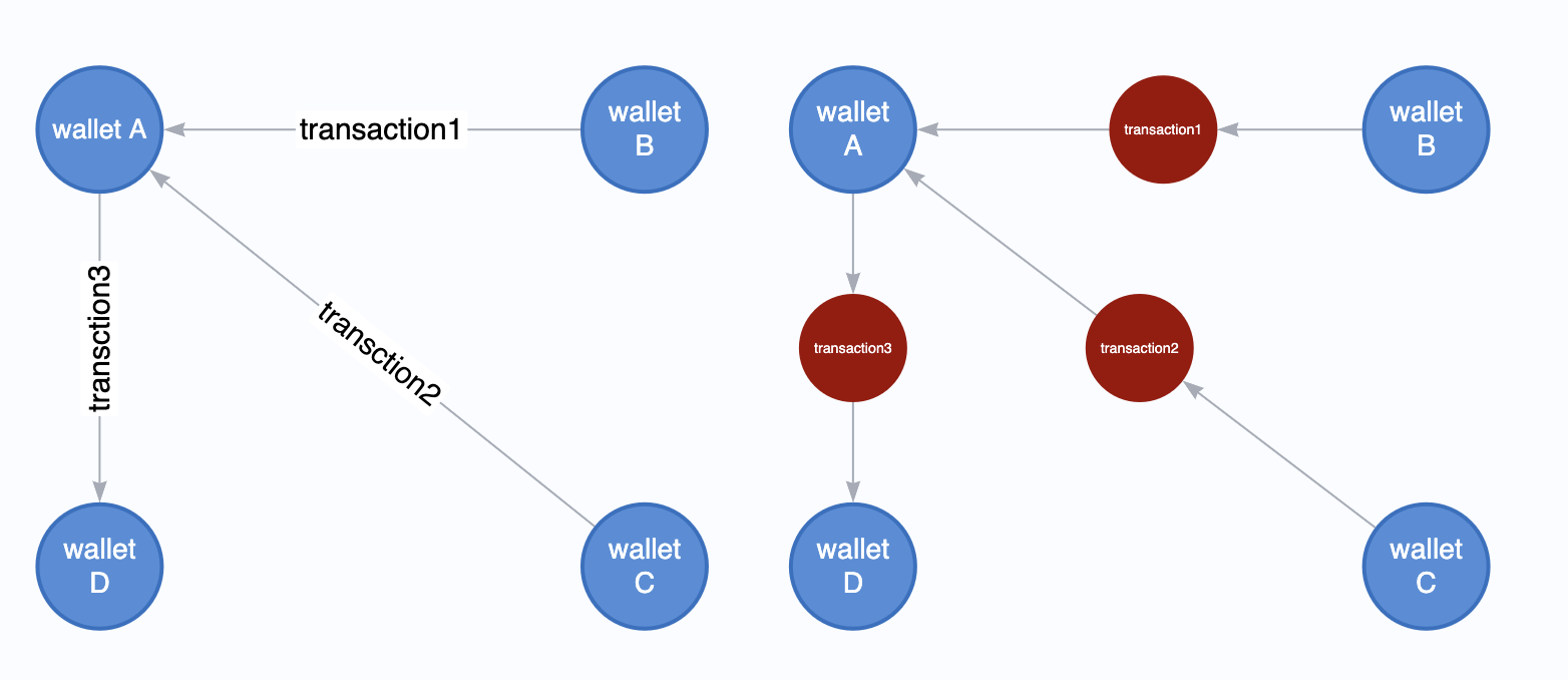
Figure 2. Financial Transaction as a Graph These two graphs show different ways of representing the same transaction graph.On the left, each trading party(”wallet”) becomes a node and each transaction becomes an edge. On the right, both trading party and transaction become nodes of different types, and edges are generated to connect them.
Processing blockchain transaction data(~11TB) into a trainable dataset is still not a miscellaneous step, due to its large size and lack of features. We experimented with different sampling approaches and feature engineerings to generate the training dataset consisting of subgraphs that aligns best with our learning object, which will be discussed in details below.
3.1.1. Node feature preprocessing via Edge Pooling
Due to the nature of decentralization and anonymity of the blockchain transactions, the nodes do not carry useful information other than its own address and account type(externally-owned account or smart contract account). Edges, on the other hand, contain the data of each transaction(value, timestamp, gas price, gas limit).
Since most of the information in the graph is stored in edges, but no information in nodes, we need a way to collect information from edges and give them to nodes for prediction. We can do this by edge pooling.[11] Edge pooling refers to the technique of collecting information from edges and giving them to nodes for prediction. This is an essential step as many GNN architectures rely heavily on node features in generating and sending messages.
Concretely, edge pooling proceeds as follows:
- For each edge to be pooled, gather each of their features and concatenate them into a matrix.
- The gathered features are then aggregated via operators such as sum, average, mean, max.
Finally, amongst the 25 node features pooled from adjacent edge features for each node, we used top 9 features selected in decreasing order of feature importance from the random forest classifier. While including all features may seem logical in training deep models, we found that we do not gain statistically significant gains by including all features, hence we decided to include a simpler set of node features in our training.
| 25 Node Features (9 selected in bold) | Description |
|---|---|
| In-degree | Number of received transactions |
| Out-degree | Number of sent transactions |
| Sum/Average/Min/Max In-value | Sum of received value in ETH |
| Sum/Average/Min/Max Out-value | Sum of sent value in ETH |
| Sum/Average/Min/Max Gas Limit | Sum of gas limit in sent transactions |
| Sum/Average/Min/Max Gas Price | Average gas price in sent transactions |
| Sum/Average/Min/Max Gas Fee | Sum [gas limit x gas price] in sent transactions |
| Average/Stdev Inter-Tx time | Average interval between transactions |
| Account Type | EOA:0, Smart Contract:1 |
While other edge features(value, timestamp) of the transaction are straightforward, there is a “gas” which is a unique component of cryptocurrency transactions. As there is no central party that clears the transactions, there must be a 1) party of workers who can publicly validate the transactions to be executed, and 2) the way to incentivize their works.
In Ethereum network, these workers are called validators. And for every transaction you want to make on Ethereum network, you must set how much gas fee you are willing to pay for your transaction to be executed. The higher you set the fee, the faster your transaction is executed, as these fees are used to incentivize the validators.
Gas fee is calculated as gas limit x gas price, and denoted in unit of Gwei(=.000000001 ETH).
Gas limit refers to the maximum amount of gas units you are willing to pay for in a single transaction. It works as a safeguard that protects users from unknowingly using a lot of gas, but if set too low, the transaction will not be executed.
Gas price is the price you are willing to pay per one unit of gas, and must be specified. It does not change the amount of gas needed to execute the transaction, hence the exact same smart contract interaction performed at different times may have wildly different price depending on the state of network congestion.
3.1.2 Subgraph Sampling
Generating a set of subgraphs that preserve the crucial local structure, and are small enough for GPU to process, is indispensable for training our GNN classifier.
One way to sample a subgraph is via breadth-first-search or a random-walk sampling starting from a set of predetermined target nodes. While they were widely used graph sampling techniques, we find it difficult to be directly applied to our task, which was to find malicious nodes via the local structures centered around them.
Breadth-first-search is a graph traversal algorithm that visits all its neighbors first, then their neighbors, and so on, exploring nodes level by level, i.e., in layers of increasing distance from the source. In our case, the size of the graph can become exponentially large when using naive breadth-first-search sampling since each node has vastly different number of neighbors.
Random-walk sampling extracts samples from a graph by simulating random walks over the nodes. In this process, a starting node is selected, and then the next node to visit is chosen randomly from the neighbors of the current node. This procedure is repeated for a predefined number of steps or until a termination condition is met. Since we needed a sampling algorithm that limits its neighbor structure up to a certain number of hops or depths, we find random-walk sampling incompatible with our goal.
Furthermore, we found that these methods ignore the temporality of the transaction which is a non-trivial trait in financial transactions. One direct consequence is that it can result in graphs that contain transactions(edges) that happened on vastly different moments, with days, months, or perhaps years of difference. Since transaction patterns of each node constantly change over time, graphs sampled in this way can contain confounding signals which can lead to inaccurate profiling. Also, each graph can have very different ages and sizes, i.e., some graphs representing 5-years of transactions records while some only containing 5-days of transactions, which again makes it challenging for our GNN to generalize.
Therefore, we decided to split the sampling stage into two:
First, split the entire transaction graphs into
This way of sampling has two inherent benefits: Firstly, it largely eliminates the potential time dependency of the transactions. Secondly, it suits the purpose of anomaly detection in realistic scenarios, where monitoring and detecting suspicious transactions should take place in reasonably short timeframe.
Neighbor Sampling The sampling begins with choosing or randomly selecting the "center" node, from which a fixed number of neighboring nodes that are 1-hop away are sampled around the center node. The process can be repeated up to the predetermined number of hops, after which a center node and neighbor nodes, along with their edges, form a subgraph which serves as a mini-batch for GNN training.

Figure 3. Neighbor Sampling [12]
Graph Saint Sampling The sampling divides the original graph into multiple non-overlapping subgraphs (or partitions) for a more manageable graph training. At each iteration, fixed number of nodes are randomly sampled from the original graph, and then form a subgraph along with their edges which serves as a mini-batch for training the GNN.

Figure 4. GraphSaint Sampling [13]
3.1.3 Transformation to Undirected graph
After generating a set of smaller subgraphs, we transform each of them into undirected graph by generating duplicate edges to be processed by GNN detector. This transformation enables the message passing to happen bidirectionally between all connected nodes, whereas in the original directed graph, message passing will only happen in the direction of incoming edges. More concretely, a center node can now aggregate information from neighboring nodes from which it received transactions, and also to which it sent transactions.
Visual comparison between message passing in directed and undirected graphs in below Figure 1 and 2.
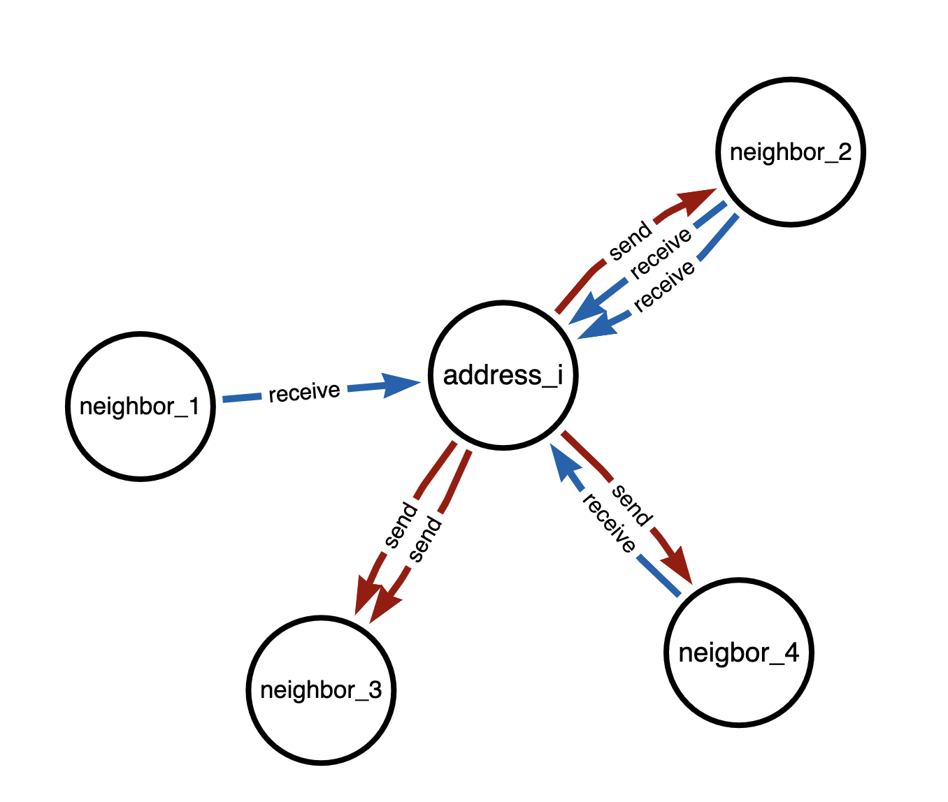
Figure 5. Directed Transaction graph
From address_i’s point of view, message passing only takes place in direction of blue(incoming) edges. Neighbor_3 signals are hence ignored, as there are only red(outgoing) edges.
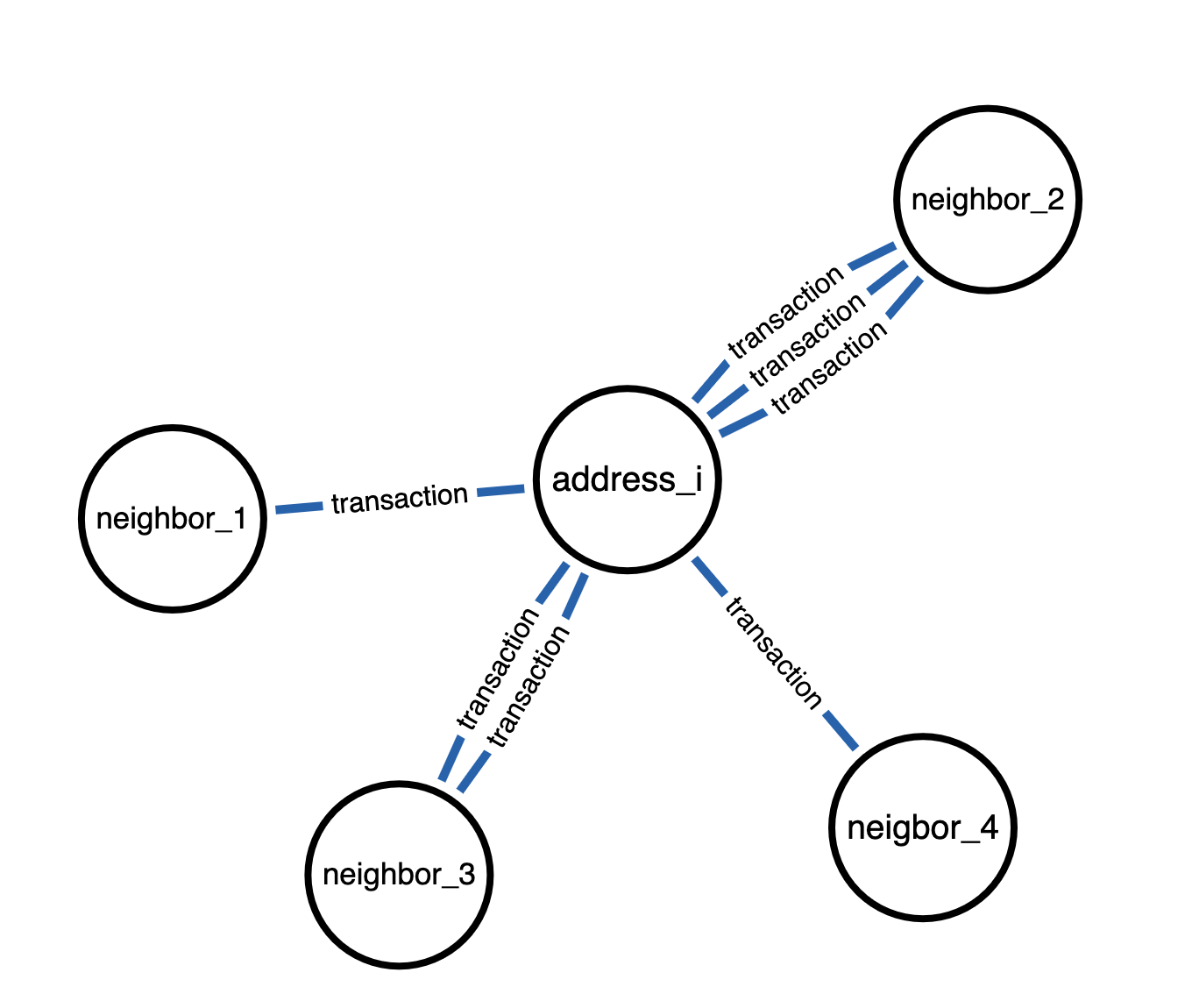
Figure 6. Undirected Transaction graph
Message passing takes place in both directions. address_i can now take signals from all adjacent nodes regardless of edge directions connecting these nodes.
3.2 Graph Neural Network Classifier
Graph Neural Network is a class of deep learning algorithms designed to directly handle graph data. Most GNN architectures use message passing to learn and update the element’s(typically, node) embedding by aggregating the information from an element’s neighbors. In essence, message passing operates much like the standard convolutional networks, where a node corresponds to a pixel, and neighbors correspond to adjacent pixels within the sliding window.
Stacking the message passing layers equals to widening its receptive field. Simply speaking, 2-layers of message passing corresponds to aggregating information from the neighbors that are 2-hops away.
3.2.1 Overview: Message Passing GNN
GNN convolutional layer updates each of the node feature vectors via aggregating the information from its neighbors, otherwise known as message passing. Key of message passing consists of
Here,
The
The
We experimented with three well-known GNNs in our classification task, which are GCN [14], GAT [15], and PNA [16], each of which differs distinctively in their
3.2.2 GNN Architectures
Graph Convolutional Network (GCN)
This architecture adopts more parameter sharing by using the same weights matrix for updating node embeddings and its neighbors.
Graph Attention Network (GAT)
Just like GCN, GAT does not distinguish between
Principal Neighborhood Aggregation Network (PNA)
This architecture uses various first- and second- order statistics, combined with three scalars linked to each node’s in-degrees, to transform neighbor messages. The messages are then concatenated and linearly transformed back to the predetermined hidden embedding dimension.
4. Experimental Details
Our goal is to find the phishing entity using the graph neural network classifier.
We define anomalous entity as either a suspicious wallet address(node) or a suspicious transaction subgraph(graph) which signals the phishing activities, and tackle each problem as a binary node classification problem and a binary graph classification problem respectively.
4.1 Dataset
The phishing account data in this article comes from Etherscan [17] which obtained the phish-tagged accounts, filtered, and deleted invalid accounts with a transaction value of zero, and finally, obtained target phishing accounts.
We first identify
Subsequently, we generate
In order to prevent the graph size from exploding, we limit the number of unique neighbors to
Finally, we have
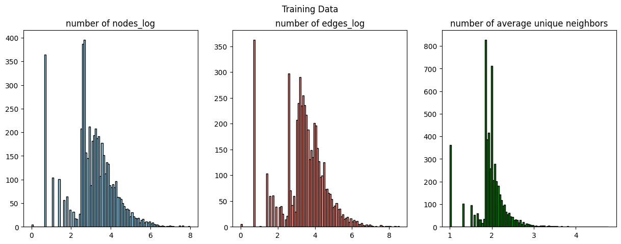
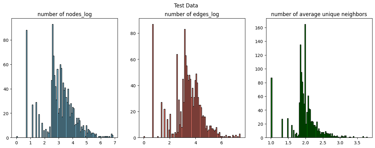
Figure 7. Distribution of Training and Testing set
4.2 GNN Classifiers
In a node classification task, GNN classifier consists of 1) 3 message passing layers, each followed by 2) batch-normalization layer except after the last layer. The updated node embeddings are then passed to 3) binary classifier layer, which is a 2-layer fully connected neural network.
In a graph classification task, we aggregate the final node embeddings by mean-pooling before passing them into a 3) binary classifier layer. The rest remains the same as the node classification model.
Message Passing Layer We experimented with three different undirected message passing layer, namely GAT, GCN and PNA. For each type of layer, we fixed the layer at depth=3, meaning each node will aggregate the information from neighbors that are maximum 3-hops away. While we avoid making these layers too deep due to the over-smoothing issue [18], we observed that 3-layers showed better performance to 2-layers, which is hence adopted in our model.
Batch Normalization Layer It is well known that one of the critical ingredients to effectively train deep neural networks is using normalization technique, such as batch normalization, layer normalization, and group normalization [19],[20],[21]. Currently, most GNNs use batch normalization, which computes statistics over a mini-batch, after the message passing layer to normalize feature representation, which we opted to use in our model.
Concretely, we put
4.3 Result
| RF | MLP | GAT | GCN | PNA | ||
|---|---|---|---|---|---|---|
| Node classification | Accuracy | 0.70 | 0.72 | 0.76 | 0.81 | 0.79 |
| F-1 | 0.69 | 0.73 | 0.79 | 0.82 | 0.80 | |
| Graph Classification | Accuracy | 0.68 | 0.69 | 0.83 | 0.97 | 0.98 |
| F-1 | 0.69 | 0.71 | 0.84 | 0.96 | 0.98 |
Table 3. Classification result
The main observations from our experiment results are in the following three aspects.
- For both node and graph classification task, GNN has consistently outperformed non-GNN baselines of random forest and MLP.
- GAT lagged behind the two other GNNs in both tasks. We suspect that this is due to the characteristic of our dataset. As the learning power of GAT comes from learning the adequate attention vector which then determines the weighting across different neighbors, it is likely that GAT failed to generalize well in our dataset where average degree is low and lot of nodes have just a single transaction record(and hence, a single neighbor). It is observed that increasing the number of heads did not help the GAT performance in our case, which also suppots the said assumption.
- Better performance in graph-level task suggests that there may be a systematic difference between the behavior of benign node involved in phishing activities and those that are not. This can be seen as a direct consequence of phishing, where benign actors under phishing attack become controllable by phishing accounts, thereby deviating from their normal transaction patterns.

cartoon: benign nodes in normal graph vs. abnormal graph
5. Discussion
Our methodology and experiments of generating transaction subgraphs considering the temporal information and scalability combined with the GNN classifier demonstrates that the graph structure benefits the task of fraud detection a lot compared to non graph-based methods. By defining the phishing detection as a subgraph classification problem, we achieved detection rate of 98% using 24-hour transaction data.
Such high success rate cannot be guaranteed in real-world scenario however, as there is a huge imbalance between malicious nodes and benign nodes, whereas our training data was constructed to remain balanced. Furthermore, the labelling of malicious nodes is potentially and likely incomplete, hence there can be a large part of anomalies left undetected. Realistically, it is also difficult to apply GNNs on the entire network of transactions in real-time, which is growing at the rate of 1M transactions per day. Possible alternative may be to put simpler pre-screening steps to filter out most of the benign entities, after which more sophisticated methods such as GNNs are applied.
Admittedly, one of the limitations of our work is that we did not fully utilize the directional information whilst transforming the graphs into undirected format(Section 3.1.3). In transaction networks, the direction of an edge is typically understood as the direction of cash flow, which is generally perceived important. While such transformation results in the loss of directional information, it also allows GNNs to pass the signals in both directions and thereby learn richer representations from all of its neighbors.
Currently, directional information could not be properly handled with most of the current off-the-shelf GNNs, while discussions over neural architectures remains nascent [23] , [24]. Therefore, in order to fully utilize the graphical structure of transaction network, designing the representation learning framework that supports directed multigraph is essential, which we aim to address in our future work.
Line Graph
To overcome the lack of original node features, another approach we considerer was to transform the graph into a line graph [25]. In line graph, also known as graph conjugate, each node becomes an edge. Then, two nodes become adjacent, or linked by an edge, if and only if they share a common endpoint. Visually, it can be expressed as below:
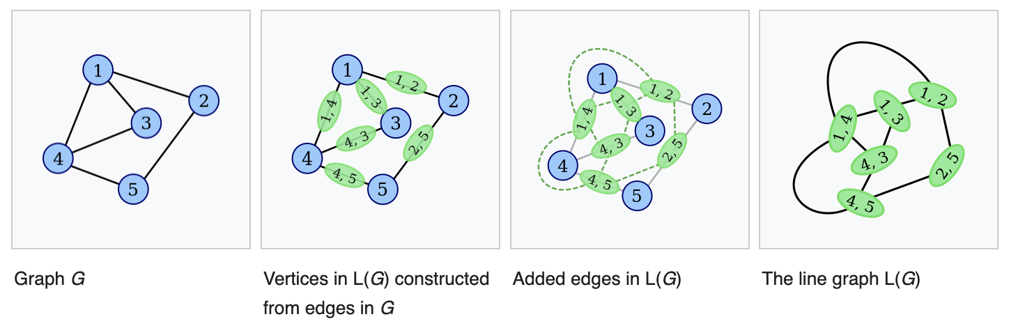
Figure 8. Transformation to Line Graph from Graph [25]
As our GNNs target to generate node embeddings, line graph of the original transaction graph, where node contains the transaction information, seemed to go more naturally with existing GNN architectures without node feature engineering.
However, the time it takes for line graph transformation was prohibitive(2+ days for 900 sampled graphs), and although our nodes now naturally contain meaningful data, 3-dimensional features(value, gas price, gas limit) were still far from enough to deploy deep models effectively.
GNNExplainer
When it comes to anomaly detection task in real-life, business units require a clear explanation as to why certain entities are classified as anomalous before making any decisions. Hence, one key hurdle when using deep learning in anomaly detection is the lack of model interpretability. Therefore, we decided to deploy GNNExplainer to add explainability to our GNN models.
Upon utilizing the explainer to our GNN classifiers however, we find that it does not give us any meaningful insights that are easily identifiable by human eyes(for instance, capturing the common transaction patterns amongst malicious graphs). In addition, some of the
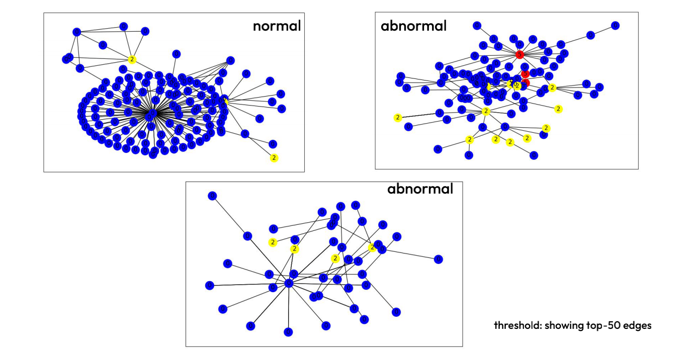
Figure 9. Example run of GNNExplainer on graph classification task
Reference
[1]
Emanuele Rossi, et al. Temporal Graph Netowrks for Deep Learning on Dynamic Graphs, 2020
[2]
Susie Xi Rao, et al. xFraud: Explainable Fraud Transaction Detection, 2022
[3]
Liu, Ziqi, et al. Heterogeneous Graph Neural Networks for Malicious Account Detection, 2018.
[4]
Hu, Binbin, et al. Cash-out User Detection based on Attributed Heterogeneous Information
[5]
Xia, Y., et al. Phishing Detection on Ethereum via Attributed Ego-Graph Embedding, 2022
[6]
Yu, T., et al. MP-GCN: A Phishing Nodes Detection Approach via Graph Convolution Network for Ethereum, 2022
[7]
Jaehyeon Kim, et al. Graph Learning-Based Blockchain Phishing Account Detection with a Heterogeneous Transaction Graph, 2023
[8]
Xiaoxiao Ma, et al. A Comprehensive Survey on Graph Anomaly Detection with Deep Learning, 2021
[9]
K.Ding, et al. Deep Anomaly Detection on Attributed Networks, 2019
[10]
X.Wang, et al. One-class graph neural networks for anomaly detection in attributed networks, 2021
[11]
https://distill.pub/2021/gnn-intro/
[12]
William L. Hamilton, et al. Inductive Representation Learning on Large Graphs, 2017
[13]
Hanqing Zeng, et al. GraphSAINT: Graph Sampling Based Inductive Learning Method, 2019
[14]
Thomas N. Kipf, Max Welling. Semi-Supervised Classification with Graph Convolutional Networks, 2016
[15]
Petar Velickovic, et al. Graph Attention Networks, 2017
[16]
Gabriele Corso, et al. Principal Neighbourhood Aggregation for Graph Nets, 2020
[17]
[18]
Qimai Li, et al. Deeper Insights into Graph Convolutional Networks for Semi-Supervised Learning, 2018
[19]
Sergey Ioffe, Christian Szegedy. Batch Normalization: Accelerating Deep Network Training by Reducing Internal Covariate Shift, 2015
[20]
Jimmy Lei Ba, et al. Layer Normalization, 2016
[21]
Yuxin Wu, Kaiming He. Group Normalization, 2018
[22]
Yihao Chen, et al. Learning Graph Normalization for Graph Neural Networks, 2020
[23]
H. Larochelle, et al. Directed graph convolutional network, 2020
[24]
Zhang, X., et al. Magnet: A neural network for directed graphs, 2021
[25]
https://en.wikipedia.org/wiki/Line_graph
[26]
Rex Ying, et al. GNNExplainer: Generating Explanations for Graph Neural Networks, 2019